0.3 — Chain rule and computational graphs

1. Why this session exists

All of backpropagation is one thing: the chain rule applied to a directed acyclic graph (DAG). If you leave this session knowing how to write the chain rule as a sum over paths in the graph, all of Chapter 2 (MLPs and backprop) becomes bookkeeping rather than mystery.

You already know the scalar version from Calc I. What we'll do here is lift it first to several intermediate variables, then to general DAGs, and finally walk through the canonical example pen-in-hand.

2. Refresher: scalar chain rule

If $y = f(g(x))$ and we set $u = g(x)$, then $y = f(u)$ and

Conceptually, a small perturbation $\Delta x$ produces $\Delta u \approx g'(x)\,\Delta x$, which in turn produces $\Delta y \approx f'(u)\,\Delta u = f'(u)\,g'(x)\,\Delta x$. In the limit, the ratio $\Delta y/\Delta x$ is the product of the two local derivatives.

Warm-up example: $y = \sin(x^2)$, set $u = x^2$, $y = \sin(u)$, so

Nothing new. But notice the structure: we multiply the local derivative at every link in the chain. This structure is the only thing that survives the generalisation.

3. Multivariable with one scalar input

Suppose now that $y$ depends on $n$ intermediates $u_1, \dots, u_n$, and that each $u_i$ depends on $x$:

A perturbation $\Delta x$ now propagates through $n$ parallel paths — one per $u_i$ — and the effects add linearly to first order:

Dividing by $\Delta x$ and taking the limit,

This is the multivariable chain rule with one input. Note its shape: a sum over links, each link carrying a product of local derivatives. This is more than coincidence; it's the special case of a much more general identity, coming next.

4. DAGs and the sum over paths

In any deep learning model, the output $L$ (say, the loss) is computed from an input $x$ through a potentially complicated sequence of intermediate operations. We represent this computation as a directed acyclic graph: each node is a variable (scalar, vector, or tensor), and each directed edge $u \to v$ indicates that $v$ is a direct function of $u$ (and possibly of other variables).

The question is: how does $L$ depend on $x$ overall? In the scalar case the answer is the sum over paths:

In words: to find how $L$ responds to $x$, walk every directed path in the DAG from $x$ to $L$; along each path, multiply the local partials along its edges; sum the results.

The proof is an easy induction on graph depth. For a node $v$ fed directly by $u_1, \dots, u_k$,

and expanding each $\partial u_i/\partial x$ recursively until reaching $x$, each term in the final expansion corresponds to one path $x \to \cdots \to v$. Applying this with $v = L$ gives the identity.

5. The computational graph as a data structure

In practice, a deep learning framework builds the DAG in two phases:

1. Forward pass. Evaluate each node in topological order from input $x$ to output $L$, storing the intermediate values $u_i$ (because they appear in the local derivatives).
2. Backward pass. Walk the graph in reverse topological order, accumulating $\partial L/\partial u_i$ at each node by summing contributions from its children. When it reaches $x$, you have $\partial L/\partial x$ ready.

Each edge carries one local partial (scalar, vector, or matrix depending on the node types); each node is responsible for summing the contributions arriving from its children. That's it.

The advantage of the graph framing over memorising chain-rule formulas is scalability: the same algorithm handles linear chains, branches, joins (multiple paths meeting at the same node), and any DAG, with no special cases.

6. Worked example: $f(x) = \sin(x^2)\cdot e^{x}$

Computing $\partial f/\partial x$ two ways: (a) by the direct scalar chain rule, as a check, and (b) by the sum over paths in the DAG, to internalise the method that will scale to deep networks.

6.1 Identifying intermediate nodes

Decompose the function into elementary operations:

$x$ appears in two places in the original formula — once inside $\sin(x^2)$ and once in $e^x$. This will become a branch in the DAG.

6.2 The DAG

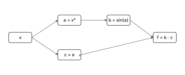
6.3 Local derivatives (one per edge)

For each edge $u \to v$ of the DAG, compute $\partial v/\partial u$ alone, treating the other parents of $v$ as constants:

Five local derivatives, one per edge. Each is trivial in isolation — that's why the method scales.

6.4 The paths from $x$ to $f$

Inspecting the DAG, there are exactly two directed paths:

6.5 Contribution of each path

The rule: multiply the local derivatives along the edges of the path.

Path 1:

Path 2:

6.6 Final sum

6.7 Sanity check via direct scalar chain rule

To validate, differentiate by the product rule and the classical chain rule. With $f(x) = \sin(x^2)\cdot e^{x}$ and $(uv)' = u'v + uv'$:

Identical. The sum-over-paths is not a different technique — it is the same chain rule, reorganised to make the combinatorial structure explicit when a variable shows up in multiple places.

7. Why this is already (almost) backprop

Look again at §6.5. To compute Path 1's contribution, we walked the edges in the direction $x \to f$ (forward mode). But notice that we could equally have walked in the direction $f \to x$ (reverse mode) and obtained the same product — multiplication is commutative. What changes is the order in which partial products are accumulated.

In reverse mode, we start with $\partial f/\partial f = 1$ at the terminal node and walk backwards, multiplying by each edge's local partial and accumulating the sum at nodes where paths meet. The result at $x$ is $\partial f/\partial x$.

The advantage of reverse mode when there are many inputs and one output (the case for every ML loss function): a single backward pass computes $\partial L/\partial \theta_j$ for every parameter $\theta_j$ simultaneously. Cost is proportional to the number of edges, not to the number of parameters. This is the asymptotic win that makes training networks with billions of parameters tractable.

We'll formalise the algorithm in Chapter 2. For now it's enough to know that backprop is sum-over-paths, computed from output to input.